Enhancing Oil Recovery Predictions by Leveraging Polymer Flooding Simulations and Machine Learning Models on a Large-Scale Synthetic Dataset
The question
Does a fast stand-in for a polymer-flooding simulator need to be a neural network?
Adding polymer to injected water can recover oil that ordinary waterflooding leaves behind. Deciding how to run such a flood means comparing many reservoir conditions, and full simulations of each one are slow. Engineers therefore train quick data-driven stand-ins, called proxy models, and earlier studies built them from much smaller datasets. We generated 163,726 simulated samples and asked which kind of model suits the task, from straight-line regression to neural networks.
What we found
The nine methods’ scores fell within a narrow band on held-out samples. A third-degree polynomial reached a test R², a measure of fit, of 0.909, performing similarly to the dense network at 0.908 and the cascade network at 0.906, while linear regression reached 0.886. Across all models, the averaged oil and water saturations were the most informative inputs.
Schematic overview
From simulated reservoir states to a comparison of nine models
Generate flow records with a simulator
Run a mathematical polymer-flooding model across parameter settings. Turn spatial flow outputs into tabular summaries, including average pressure, fluid saturations, and polymer concentration.
Add noise and separate test records
Perturb the data with artificial noise, then randomly reserve 30% of records for testing. The remaining data support training, tuning, and neural-network validation.
Compare several kinds of prediction model
Train linear and polynomial models, tree-based methods, and two neural networks. Compare their test errors and examine which input variables their predictions depend on.
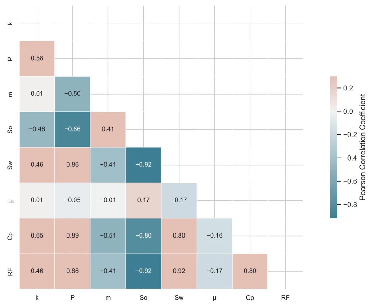
What information the records contain
Each numbered cell measures how two variables vary together after noise is added. RF is recovery; Sw and So are water and oil saturation. Their strong relationships with RF help explain why these reservoir-state summaries are informative inputs.
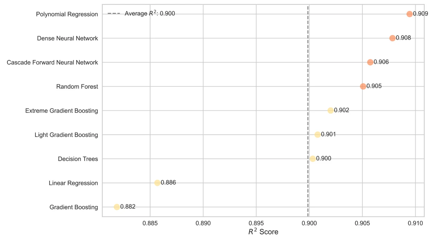
How all nine methods compare
Each dot is a model’s reported test R². Further right means a better fit to the held-out recovery values. Polynomial regression and the two neural networks are close. All nine scores lie between 0.882 and 0.909.
Figure details and test conditions
The dataset has 163,726 simulated records and seven inputs: permeability (k), pressure (P), porosity (m), oil saturation (So), water saturation (Sw), oil viscosity (μ), and polymer concentration (Cp). Spatially varying simulator outputs are averaged into records. Added Gaussian noise has zero mean and a standard deviation of 30% of each column’s standard deviation. Testing uses a random 30% split from this synthetic dataset. R² measures fit relative to predicting the mean; 0.909 is not 90.9% accuracy.
Figure 3, PDF page 6; Figure 10, PDF page 17 from the paper (opens in a new tab)
Using proxy models to explore polymer-flooding scenarios
Polymer flooding is a preferred tertiary recovery method once conventional waterflooding becomes less effective. Its results vary widely: a review of 55 projects at China’s Daqing field found incremental recovery between 1.9% and 19.5% of the original oil in place. That review linked the outcome to polymer properties, well configurations, and other operating choices. Simulating such choices takes extensive computing time, because each run must handle porosity, permeability, and multiphase flow.
Data-driven proxy models are increasingly used to evaluate operating scenarios quickly instead. The earlier chemical-flooding studies we reviewed used much smaller datasets, such as 202 experimental data points or 624 simulations. We wanted to understand how well machine learning could capture the relationships in data covering a much wider range of conditions, and which model family would suit that task. The comparison therefore included parametric and non-parametric methods, ensembles, and neural networks.
Building the dataset
We solved a Buckley–Leverett model of polymer flooding across a range of reservoir parameters, producing 163,726 samples. The model’s outputs for pressure, oil and water saturation, and polymer concentration vary across the reservoir, so we averaged each one to fit a table. With permeability, porosity, and oil viscosity, that gives seven inputs. The target is the oil recovery factor, the fraction of the original oil recovered.
Models trained on the noise-free table reached near-perfect scores. Synthetic data lack the distortions of real measurements, so we added Gaussian noise with a standard deviation of 30% of each column’s own spread. We then held out a random 30% of samples for testing.
Comparing nine prediction methods
We compared nine methods, ranging from linear regression to decision trees, boosting methods, and two neural networks. Their test scores fell within a narrow band, with a third-degree polynomial performing about as well as the dense network and linear regression also coming close. Random forest fitted its training data best (R² 0.971) but scored 0.905 on the test set.
Permutation importance shuffles one input at a time and measures how much a model’s score drops. In every model, oil and water saturation mattered most and polymer concentration came third. Permeability, porosity, and viscosity mattered least.
Scope of the study
The inputs include averaged saturations computed by the simulator during the flood. Before noise was added, the recovery factor was perfectly correlated with water saturation (1.00) and with oil saturation (−1.00). The task is therefore to estimate recovery from a simulated flow state, not to forecast it from properties known before injection. All samples come from one simplified model, and testing a real-field dataset with more parameters is the next step.
Methods and scores
Test R² values: polynomial regression 0.909, dense network 0.908, cascade-forward network 0.906, random forest 0.905, extreme gradient boosting 0.902, light gradient boosting 0.901, decision tree 0.900, linear regression 0.886, and gradient boosting 0.882. The classical models use a 70/30 training/test split. The neural networks also reserve 30% of their training share for validation.